Categories
HSQL

Week 12: Dedup & Documentation (& Examples)

This week focused on finishing up documentation, a little bit of cleanup and one final task of implementation that would be helpful.

DISTINCT

The SELECT DISTINCT clause currently uses a DEDUP(x,ALL), which is notoriously slow for large tasks. Instead an alternative clause was suggested

TABLE(x,{<cols>},<cols>,MERGE);

//eg. for a t1 table with c1 and c2
TABLE(t1,{t1},c1,c2,MERGE);

This looks good!

But, the question is – how to get the columns c1 and c2 for the table t1? It may not always be known, or worse, the known type information may not be complete. Here, we are presented with two ways in which we can proceed with this information:

  1. Stick with DEDUP all the time. It is slow, but it will work.
  2. Use the new TABLE format, falling back to the DEDUP variant if type information given is not sufficient.

This is great, and it also incentives typing out ECL declarations, but it still feels as a compromise.

Template Language

Everything changed when I realised that ECL has a wonderful templating language. For a quick idea on what the point of a template language is, it can be used in a way similar to the preprocessor directives in C – macros that can be used to write ECL.

So, what can we do here? The good thing about writing macros is that since they are based off the same solution, the macro processor can work with data types in ECL very well, and also, can make ECL code.

So, can we write an expression that creates the c1,c2 expression, given that the table t1 is given?

__dedupParser(la):= functionmacro
    #EXPORTXML(layoutelements,la);
    #declare(a)
    #set(a,'')
    #for(layoutelements)
        #for(field)
            #append(a,',');
            #append(a,%'{@label}'%);
            #end
        return %'a'%;
    #end
endmacro

Although I won’t go into the details of this interesting function macro (A macro whose contents are scoped), in essence, it can take a record, and put out a snippet of code that contains the columns delimited by comma.

Using __dedupParser

Although the naming isn’t accurate, we can inspect what the macro does by an example

Given a record R1, which contains two fields, f1 and f2 (Assume both as integer), then __dedupparser(r1) will create an ECL code snippet of “f1,f2,” (Notice the trailing comma). This works nicely with the RECORDOF declaration, which can help get the record associated with a recordset definition.

So, this brings something really useful, as we can now have this general code syntax –

TABLE(<t1>,{ <t1> }#expand(__dedupParser(RECORDOF( <t1> ))),MERGE);

This simple expression generalizes the entire TABLE function pretty effectively.

Adding this into code, it is important to remember that the function macro needs to be inserted separately, and most importantly, only once in a ECL file. This is better done by tracking whether a DISTINCT clause has been used in the program (Using an action like we had done earlier), and inserting the functionmacro definition at the top in this case. And with this, a good new improvement can be made to the SELECT’s DISTINCT clause.

Distinct now has shinier code!

This should perform much better, and work more efficiently.

Documentation

So far, some of the syntax was stored and referred personally by the use of notes, memory and grammar. Writing this down in essential as a way of keeping a record (More for others, and even more importantly, for yourself). So, keeping a document to denote the syntax available to the user is rather important.
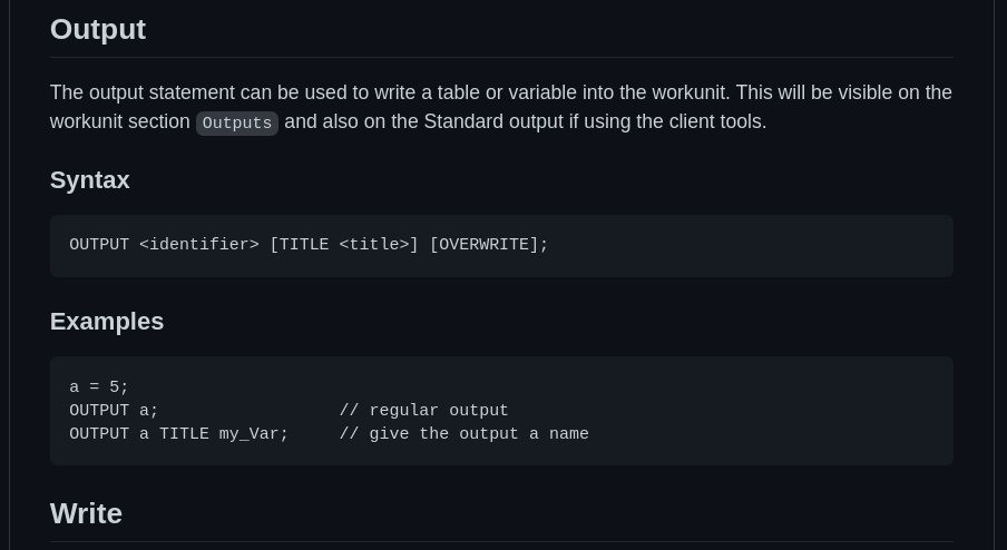
Docs for OUTPUT!

Here, its important to lay out the syntax, but also present some usable examples that an explain what is going on with that code segment. (Yeap, for every single statement!)

Winding up!

With documentation, that ends a lot of the work that was there. In fact, its already Week 12, although it is still surprising how quickly time has passed during this period. My code thankfully doesn’t need extensive submission procedures as I was working on the dev branch, and work will continue on this “foundation”. It has been a wonderful 12 weeks of a learning and working process for me, and I would like to thank everybody at the HPCC Systems team for making it such an enjoyable process! Although this is all for now, I can only hope that there’s more to come!
Categories
HSQL

Week 11: Machine Learning Methods and Final Presentation

This week, was adding some more Machine Learning Methods, and a final Presentation for the work I’ve done through this period!

Adding More Machine Learning Support

A set of other

A set of other training methods were also added. GLM was decided to be split into some of its more commonly used components. This expands the support to also include:

  1. (Regression) Random Forest
  2. Binomial Logistic Regression
  3. GLM
  4. DBScan
More model types!

This, is rather easy to do now that we have added declarations; there is a standard ML_Core.dhsql memory file, and this provides a nice way to provide built-in declarations.

Going from here, following the declaration syntax, we can add in a lot of the methods:

Here is a declaration for Classification forest

Predict-only methods

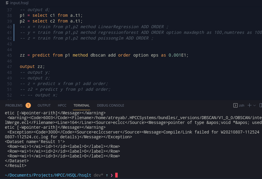
DBScan is a good one, as it is an unsupervised Machine Learning technique that does not fit into the traditional ‘train-predict’ idealogy. Here, the idea is have a variant of the predict statement that captures a syntax similar to train. Let’s model the statement as:

predict from <ind> method <methodtype> [ADD ORDER] [<trainoptions>];

Adding in the grammar, as most of the work is similar to train, we can add this in, and voila! A new statement for this form of machine learning!

DBScan!

Final Presentation

This is where a lot of the time was spent; I’ve been gathering and making examples for HSQL, and how it can be used, and on Thursday, we had a presentation on HSQL, what’s new and how it can be useful! (I will post more about it when I can!)

Wrapping up

As week 11 comes to an end, there are some things that may require documentation, and those are being looked at; and that’s about it! We still have to add some examples for the easy to use machine learning statements, and maybe also look at some code generation suggestions. (and perhaps even try to implement one!)

Categories
HSQL

Week 10: Train and Predict

This week’s focus was more on getting train and predict working, the last two remaining statements. There were also some minor bugfixes.

Declarations

Declarations are used on the .dhsql files that we’ve worked on in the past. They’re a really nice candidate for adding in a way for bundles to indicate their train methods. However this time around; the ML_Core bundle is auto-loaded on import, but the actual machine learning methods are separated into many different bundles. Let’s see what’s need to actually make the machine learning statement work-

  1. The training template
  2. The prediction template
  3. The return type of the train statement
  4. The return type of the predict option
  5. Is discretization required?
  6. The model name (When predicting)
  7. The additional options that may be passed to train
  8. Are there any other imports?

So that’s 7 things that’s required. We can wrap it up into a whole declaration statement that the user need not worry about, but just expressive enough to list these.

From here, let’s take an example for LinearRegression to go about it.

declare linearregression as train '{bundleLoc}{ecldot}OLS({indep},{dep}).getModel' REAL RETURN TABLE(int wi,int id,int number,real value ) WHERE '{bundleLoc}{ecldot}OLS().predict({indep},{model})' RETURN TABLE(int wi,int id,int number,real value ) by LinearRegression;

That’s a lot but what does it mean?

  1. LinearRegression is an available training method.
  2. It uses {bundleLoc}{ecldot}OLS({indep},{dep}).getModel as a template to train. The appropriate code gets filled in as required. (Yes, the ecldot becomes a ., this is just to help with in-module methods, which may be a thing later but not right now).
  3. REAL – it does not require discretization.
  4. RETURN TABLE(int wi,int id,int number,real value ) – The model is shaped this a table. It can also just be RETURN ANYTABLE if the shape is too annoying to list out or not required.
  5. WHERE – switch over to the details for the prediction part
  6. '{bundleLoc}{ecldot}OLS().predict({indep},{model})' – This is the template to predict with
  7. RETURN TABLE(int wi,int id,int number,real value ) – The final result looks like this!
  8. The method needs an import of LinearRegression to work.

Why are there two ‘return’s? That is because the model is not going to look like the prediction, and often, many machine learning methods give different shaped predictions (E.g. Logistic Regression returns a confidence too along with the result).

Adding these in, we get some good news of it working (Debugging is a god-send in Javascript programs, and VSCode’s JS Debug Terminal really makes it so much easier!). No outputs and screenshots yet though, there’s still some work left.

Tag Store

This is a good time to remember that there should be a way to tag variables in the variable table so that some information can be drawn out of them. Why is that useful?

Well, let’s take an example

  1. Easily find out which layout the table originated from.
  2. Tag a model (which is basically a table), as made with an ‘xyz’ method (eg. by LinearRegression)

This is actually easy. We can write up a simple Map wrapper and provide a way to pull out strings, numbers and booleans:

private map: Map<string, string | number | boolean>;
constructor() {
    this.map = new Map();
}
getNum(key: string): number | undefined {
    const entry = this.map.get(key);
    if (typeof entry === 'number') {  // only return numbers
        return entry;
    } else {  // dont return non-numbers
        return undefined;
    }
}

We can extend this for the other types also! Now to keep a track of the keys, we can have a nice static member in the class:

static trainStore = 'trainmethod' as const;

Instead of having to remember the string, we can use this static const variable as well. We could also implement a whole type system and only allow specific keys, but that’s way too complex for a simple key value store.

Adding this as an element for our base data type DataType, we can now have a small k-v pair set for the variable tables. Note that here, WeakMaps were also a good way of doing this, but I do not wish to worry about equality of data types yet.

Train

Baby steps, and we are getting to Train. Passing the required arguments into train, the general way of generating the AST for the train node goes like –

  1. Find the train method. If it doesn’t exist, its time to throw an error.
  2. Check if the independent and dependent variables exist, and if they do, warn if they’re not tables. (Throw a huge error if they don’t exist to begin with.)
  3. Now, check the train arguments/options. Map the argument names with the datatypes and if the user has supplied them. If there has been a repeat passing of the same argument (name), or that given argument does not exist, throw an error.
  4. Dump all this information into the node, and done!

Doing all this, the code generation steps become easy! Just stack the variables (Similar to SELECT, discretize and add sequential ids if required, and fill it into the code template), and we have train!

Three days of effort and I can finally say that 2 = 1*1+1! (/s)

Predict

Predict follows a similar pattern – find the method, check if the arguments to it are tables, and then proceed to fill in the templates and the required steps using the stacking method from SELECT. Not going into a lot of detail as its the same, but here’s another thing.

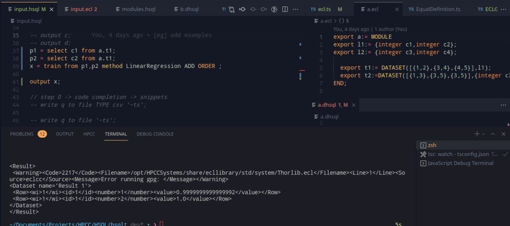
We can use the tag store, and find the original model type, and this makes mentioning the model type optional. This allows for this nice pretty syntax!

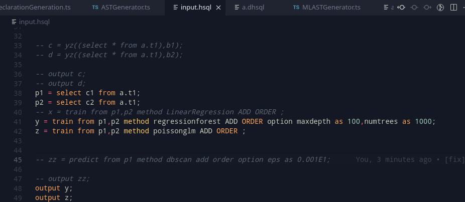
Train, Predict, and code generation!

Of course, If you are keen enough, I have used incompatible train and predict templates (Classification and Regression Forest). This was just a way to check that by mistake, the same template wasn’t being used. This was fixed, and we now have LinearRegression, and Classification Forest as well! (2/?? done!)

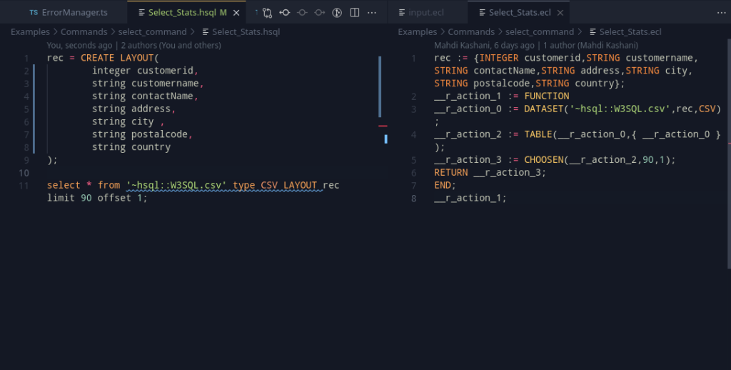
Offset

I realised there was still something in SELECT that needs to be worked on – loading data from logical files.

The syntax currently looks like this

SELECT * from '~file.csv' TYPE CSV layout l1;

Now, in ECL, a common pattern is to use

DATASET('~file.csv',l1,CSV(HEADING(1)));

This removes the header part. The best way, for us is to use the offset clause. But, currently, it is only allowed a suffix to the limit clause. To deal with this, we can make this both optional.

However, the code generation stays almost the same, except for if only offset is specified. In such a case, we can fall back to using a array subscript method.

For example, offset 1, can translate to [1..]. This works well, and gives us a nice output!

Can you spot a mistake in the offset code?

There’s one small issue though. ECL arrays are 1-indexed. In this case, its trivial too, we can just add a 1, and it’ll work perfectly.

offset 1 hence, should actually become [2..].

Winding up

This completes this week 10 too, and we’re almost there! Now, we can move towards week 11, with the following plans –

  1. Prepare for the final presentation next week
  2. Add more training methods!
  3. Maybe look around and find some nice ways to show the documentation and information about this project. Typedoc is already present in the project, but perhaps Docusaurus or Gitbooks would be good to use!
Categories
HSQL

Week 9: Lots of things!

This week has been a big week – extending SELECT to load up datasets from logical files, modules, functions, and running from a CLI was worked on. There’s a lot to uncover!

Select from dataset

As layouts have now been introduced, one handy way of using select can be added in – loading up a dataset. The idea behind it is similar to how join works in HSQL – a new aliased variable that contains the necessary table. The shape of the table may be made out from the layout that was supplied to the command. Consider the following example:

Select * from '~file::file.thor' layout l1;

This above example selects from the logical file using the layout l1. To see how this would translate to ECL, we can take the following example as what we want to achieve –

__r__action_x :=FUNCTION
  src1 := DATASET('~file::file.thor',l1,THOR);
  res := TABLE(src1,{src1});
  return res;
END;
__r__action_x; // this is the end result-> assign it if needed

Taking a look at SELECT, we can add support for ECL’s 4 supported types – XML, JSON, CSV, THOR. THOR is relatively easy to work with, but CSV files very commonly need to have their headers stripped (CSV(HEADING(1)) more precisely, when writing the ECL Code). This, might be a good point for SELECT’s offset clause to fit in. Currently it can only work with limit, but that restriction can be lifted later (by falling back to array subscripting).

Adding this SELECT Dataset as a separate node for the AST, we can treat it just like a join, and voila!

We can select from a dataset!

Modules

Modules are a great way to represent and structure code. Thankfully, as we’ve worked with select, the modelling style is similar here. The variable table entry for modules already exist, so its just a matter of adding in the right syntax. A good one to start would be

x = create module(
  export k = 65;
  shared j = 66;
  l = 67;
);

Currently the grammar still includes ECL’s three visibility modes, but we will look at that later.

When creating an AST node, we can create a new scope, and put our new variables in to create the module before popping them off to create the module entry; and while I thought this was easier, this was more of a “easier said than done”. However, thankfully, it didn’t take much longer since as I had mentioned, the data types were already in place.

And… modules!

The variable table (or symbol table in regular compiler literature) can already resolve by the dot notation, so the type checking it works seamlessly and translates identically without any problems to ECL.

Functions

Functions are intended to be a nice way to reuse code. Implementation wise, they look pretty intimidating. How to start?

Well, let’s start at the grammar

create function <name> ([args]){
  [body];
  return <definition>;
};

This is something to start with; it looks simple to work with and implement for the grammar. Going into the specifics, we can look at the arguments – there can be two types – the usual default primitive arguments, and a table. For the former, the standard C type rules work, for layouts, we can define them somewhat like this example:

create function yz(layout l1 x,int y){
  //...
};

So, an important thing here, is to actually resolve this layout. Once we realise the layout, we can work with AST generation for the function in a way similar to that of the select statement – we can push a new scope into the function, and thankfully, as ECL supports variable shadowing for functions, we can push in the arguments as variables into the scope. Once that is over, we can pop the scope, and the resultant variables are gone! The arguments and the result type needs to be stored by the datatype though, and a function needs to be represented in the variable table too.

Adding all this in, only does half the job. Now that there’s functions, there needs to be a way to call them.

Function call

Function calls are rather important to be able to execute them. Now, the easiest is to model it after most of the programming languages:

x = somefunction(y,z);

This function call can be checked during the AST Generation steps by the following steps:

  1. Locate the function from the variable table. If it cannot be found, throw an error.
  2. Match the function arguments. Does the length and the types match? If no, throw (lots of) errors.
  3. The function call node evaluates to the return type of the function now.

From here, the assignment node takes care of the returned type from there.

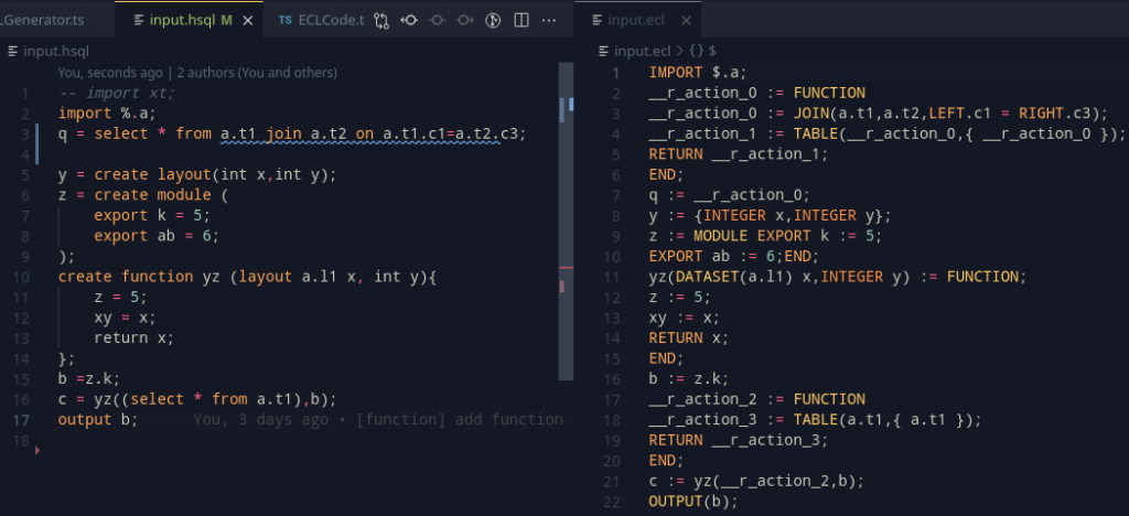
Adding all these steps, we can get something marvelous –

Functions and Function calls! Finally (The example also shows passing a select statements results into the first argument)

Running

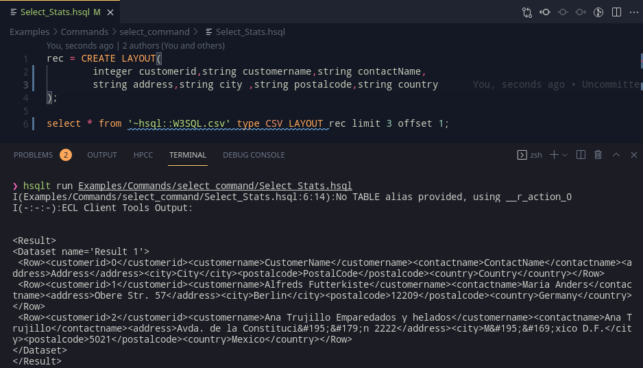
HSQLT already consults eclcc for getting the paths; this is a good opportunity to use this functionality to extend this and use ecl to compile and submit the resultant .ecl program. After checking if the outputs were produced from the previous code generation stage onto the filesystem, we can take the mainfile which stores the entry point for parsing, and submit that file’s ecl program to the cluster using the client tools. Using some nice stream processing, we can project the stdout and stderr of the child ecl process and get this nice result:

An easy way to run the programs now!

And there’s still more to go. Going over to the extension:

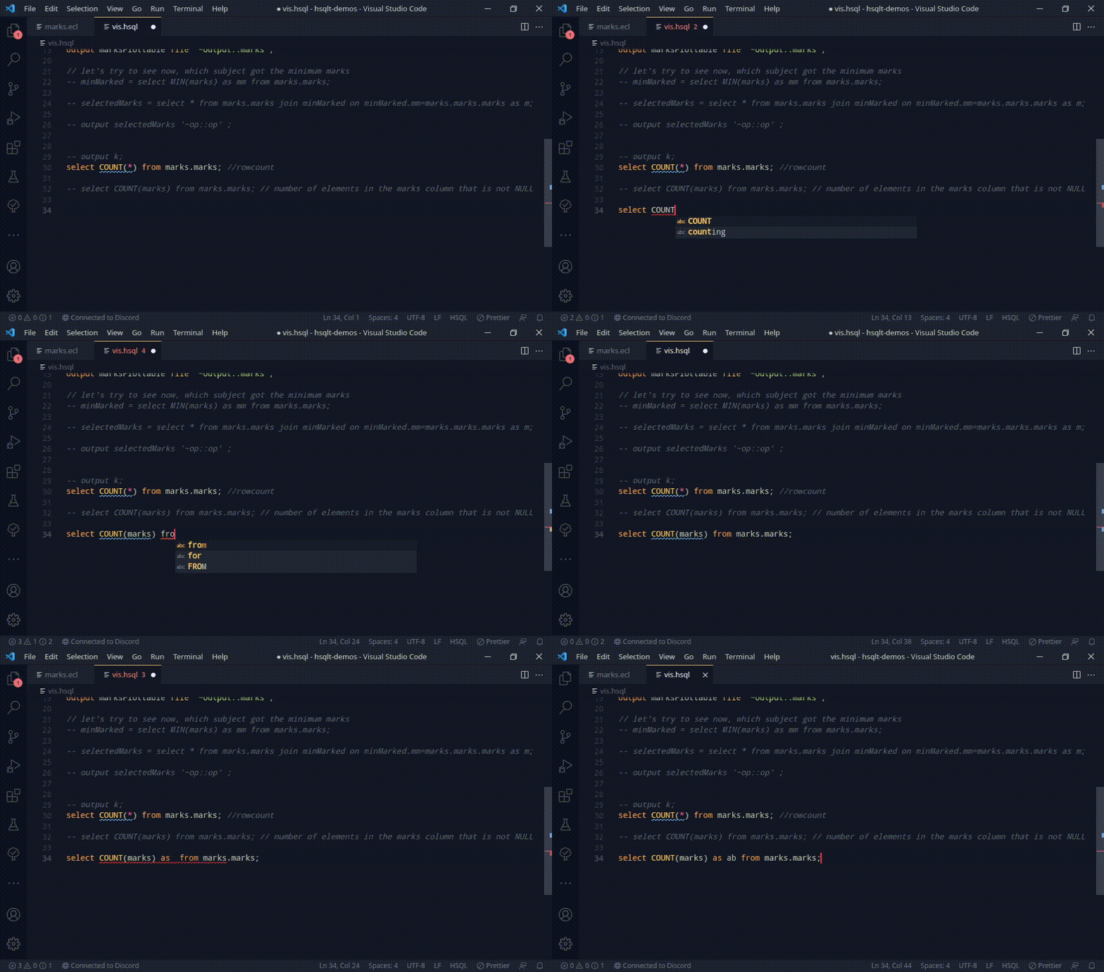
Code completion – Snippets

Snippets are an easy way to work with programs. VSCode snippets are a first step towards code completion. The example below can be typed with a simple write and the line will be filled in. Using TAB, the statement can be navigated and the appropriate sections can be filled in.

Write Snippets

Code completion – Variable Resolving

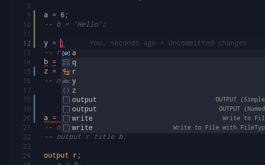
Variable resolving can be combined with Snippets to allow the user to write programd faster and more effectively. Pressing Ctl+Space currently brings up the current program’s table for auto complete. This, can be added by storing the last compilation’s variable table, and using that to find the possible variable entries.

We can see the variables!

Wrapping up

Oh dear, that was a lot of things in one week. The plans for the next week can roughly be summed up as –

  1. Look into implementing TRAIN and PREDICT statements for Machine Learning.
  2. Look into code generation, fix any glaring issues that result in incorrect code generation.
Categories
HSQL

Week 8: Export, Layouts and Syntaxes

This week was focused on creating EXPORT/SHARED to work, and to add over importing from current directory and Layouts.

Exports

Exports are a very useful feature in any language. The main idea here is to export some data and layouts, that can be reused in another module. Taking a piece from ECL, we can define two such export modes: SHARED and EXPORT. Let’s take a look at the example below:

export x = select * from table1;
export y = select * from table2;

This should export out x and y so that it may be used outside. A key note to be made is that unlike ECL, the export <filename> := MODULE should autowrap the program.

There are two possible ways of solving this. One is to write a visitor that can decide whether there is a need to export the module, or we can offload the work to the parser, using a grammar action.

Consider the following simplified grammar:

program: (stmt SEMICOLON)* EOF;
...
stmt:= scope IDENTIFIER '=' expr;
scope: EXPORT|SHARED|;

This above grammar accepts a scoped definition. Instead of doing the computation on the visitor/AST Generation side, we can use locals to get this value by the end of the parsing process itself.

program locals[willExport:boolean=false]: (stmt SEMICOLON)* EOF;
...
stmt:= scope IDENTIFIER '=' expr;
scope: EXPORT { $program::willExport:boolean=true} | SHARED { $program::willExport:boolean=true} |;

This is a quick and easy way to set the program to decide whether it will be wrapped as a module.

Proceeding further with this, this setup does yield an interesting use – since the variable names in an exported ECL module is the same as that of the window, we can actually import translated hsql files from an ECL file and use it the same way!

Imports from the current directory

ECL has a $ operator which can be used in imports to refer to the current directory. Although grammar support has been there for it in HSQL, the compiler would read and only use the % operator (which performs the work of the $ operator from ECL) as an indication for whether the standard libraries could be skipped or not.

This implementation requires proper file location information is passed into the AST Generator, which allows us to Import modules as required. This also adds support for detecting cyclic imports (which are not allowed in ECL either). This can be added in via the presence of an include stack.

The idea of an include stack, is to present a stack, where the top of the stack will represent the current file being processed. Once this is over, the file is popped. Hence, to detect an include cycle, it is trivial to check if the file is already present in the current include stack.

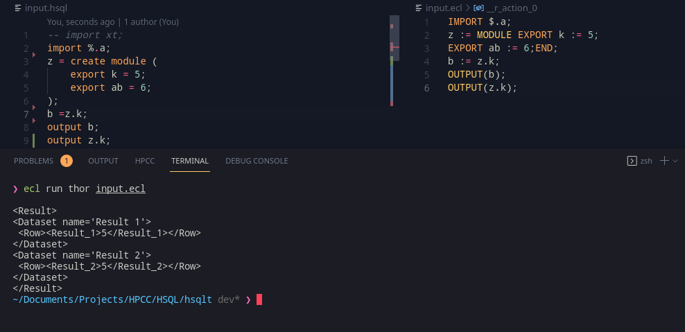
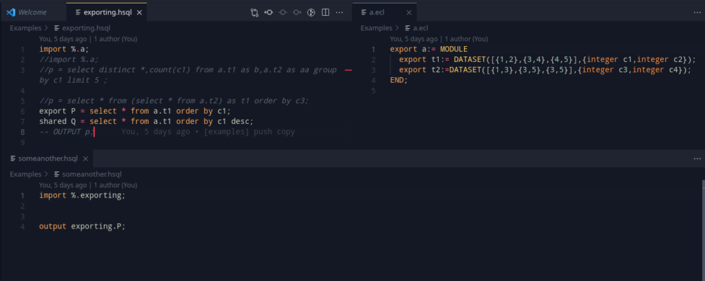
Adding all this in, we get a nice example that summarizes the work:

Exporting!

Layouts

From here, the work shifted onto layouts. Although not explicitly a goal, layouts are an important precursor to functions and for select. Looking at the syntax of the CREATE TABLE syntax in SQL, we can work with and add a layout with an example syntax as:

x = create layout(
  int p, string q
);

The data type is kept in the front to allow people from other languages to be familiar with it (Hint: C/C++/C#/Java/JS)

Internally, a layout represents a RECORD. After adding them in, they look somewhat like this:

Layouts

Layouts are represented in the Variable Table (Commonly referred as symbol tables in usual compiler terminology) as their own separate term, and can be used to create tables. This, is actually thankfully trivial as the contents of a layout are identical to that of a table, Col elements. With a deep clone of its children, we can create a corresponding table. This will come in use as more features get added into the language.

Wrapping up for the big week ahead

There were some key precursor elements that were made this week, and the syntaxes of Module and Function have been defined, and the idea is to start working on them from here on out. The rough plan for next week is-

  1. Work with layouts
  2. Add in modules
  3. Add in support for functions
  4. Prepare some more examples for showing the functionality of HSQL.
Categories
HSQL

Week 7: WRITEs, DISTRIBUTE and Bugfixes

This week’s work was on getting the WRITE statement to work, and extending a DISTRIBUTE extension to SELECT. The rest, was getting some bugfixes and reading.

Write

The OUTPUT statement in HSQL is intended to be a way to output values to a workunit. In ECL however, OUTPUT can be used to write to a workunit as well as to a logical file. In HSQL, it is better to bifurcate the process into two separate commands. With this, the idea behind the WRITE statement, is to allow writing datasets into the logical file.

The syntax for WRITE was designed as:

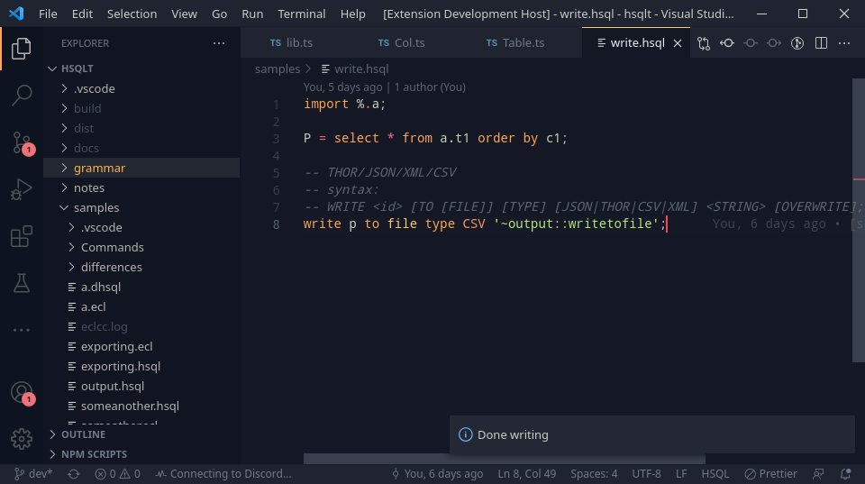
WRITE <id> [TO [FILE]] [TYPE] [JSON|THOR|CSV|XML] <STRING> [OVERWRITE];

ECL can support outputs of 4 types – ECL, JSON, THOR, CSV. Typescript enums are a great way of supporting this:

export enum FileOutputType {
    THOR,
    CSV,
    JSON,
    XML,
}
// get the enum value
const y = FileOutputType.THOR;
// y is 0

// get the string
const z = FileOutputType[y];
// z is 'THOR'

The enums provide a two way string and integer conversion; which is convenient for storing the two representations while still being good computationally.

Adding in the AST and Code generation stages, we can test out some examples:

-- hsqlt make Commands/write_command/write.hsql
import %.a;

P = select * from a.t1 order by c1;

-- THOR/JSON/XML/CSV
-- syntax:
-- WRITE <id> [TO [FILE]] [TYPE] [JSON|THOR|CSV|XML] <STRING> [OVERWRITE];
write p to file type CSV '~output::writetofile.csv';

-- to thor files
write p to file type THOR '~output::writetofile.thor';

-- to xml
write p to file XML '~output::writetofile.xml';

This gives a nice way to write files to output so they can be used outside too.

DISTRIBUTE extension of SELECT

DISTRIBUTE in ECL is used to distribute data across nodes, for further computation; it is really helpful for managing data skew as we go along with further computations.

The idea for it is to be added as an extension in the HSQL select statement with the grammar being:

DISTRIBUTE BY <col1>[,<col2>,...]

This will add a DISTRIBUTE element to the end of the SELECT pipeline which will aid in managing data skew.

a = select * from marksmodule.marksds where marks>40 distribute by marks,subid;

The output for this expression looks like this:

__r_action_0 := FUNCTION
__r_action_1 := marksmodule.marksds( marks > 40);
__r_action_2 := TABLE(__r_action_1,{ __r_action_1 });
__r_action_3 := DISTRIBUTE(__r_action_2,HASH32(marks,subid));
RETURN __r_action_3;
END;
aa := __r_action_0;

The __r_action_3 is a computation that obtains the distributed definition and this is returned in that context. HASH32 has been recommended for use as per the documentation when distributing by expressions/columns, and was chosen as it would be the most used way of distributing that still maintains even distribution.

Bugfixes for the extension

Seems like the extension was lagging behind HSQLT. This is from the previous update that added in the file system reading. As the file locations have to now be provided separately, the Extension had not yet been configured for it. Additionally, the extension’s client and servers work on different folders. Due to this, the server can successfully locate files, whereas the client fails to. This required support for the compiler to refer to another directory ‘offset’ from the current directory (This has been added to the CLI tool as a -b flag).
Adding this and support for %, allows HSQL to be used with the extension a bit more easily.

Writes, clean outputs and no more ‘Warnings’!

Demo

As there was a demo that was done at the end of this week, various examples have been created to show how HSQL may be used. Currently, they do not showcase actual usecases, but only the syntax and the usability of the language. Nearly all supported features have been enumerated and the plan is to have a nice set of examples for each statement going ahead. The demo actually revealed some good to have feedback and the plan is to work towards getting some more statements and features as we go along.

Wrapping up

As Week 7 is coming to wraps, the plan is to work on these for Week 8:

  1. Add support for exporting definitions
  2. Add support for bundling definitions into modules in HSQL
  3. Look into procedure syntaxes in HSQL
  4. Evaluate existing featureset and make some examples to work on performance and correctness.
Categories
HSQL

Week 6: Plots and TextMate Grammars

This week’s plans were to essentially work on and implement the PLOT statement, and then to see how to update the TextMate Grammar and add in the new syntax.

Plots

Continuing from last week, we have auto-imports and an AST for Plots. With some little code generation, we can have a functioning PLOT statement.

Here’s the implementation I ended up choosing out of the 3 possible ways:

PARALLEL(OUTPUT(,,NAMED('<name>')),<module>.<function template>);

PARALLEL allows for the actions to be executed in parallel, or rather, parallel given the best ordering that the ECL Compiler finds.

The code generation section was added in using this above idea, and care was taken to not emit the plot statement if the plot method was not found (and also raise an error) – as in such a case no template for the function call would be found.

Let’s take this sample code for reference

import marks;

-- lets get all the average marks of each subject
counting = select DISTINCT subid,AVG(marks) as avgmarks from marks.marks group by subid;
// join this to get the subject names
marksJoined = select * from counting join marks.subs on counting.subid=marks.subs.subid;

output counting title marksAvg;
// filter out what we need for plotting

marksPlottable = select subname, avgmarks from marksJoined;
// some different plots
PLOT from marksPlottable title hello type bar;
PLOT from marksPlottable title hello2 type bubble;

Doing some sample codegeneration after implementation, we get this translation:

IMPORT Visualizer;
IMPORT marks;
__r_action_0 := FUNCTION
__r_action_1 := TABLE(marks.marks,{ subid,avgmarks := AVE(GROUP,marks) },subid);
__r_action_2 := DEDUP(__r_action_1,ALL);
RETURN __r_action_2;
END;
counting := __r_action_0;
__r_action_3 := FUNCTION
somesource := JOIN(counting,marks.subs,LEFT.subid = RIGHT.subid);
__r_action_4 := TABLE(somesource,{ somesource });
RETURN __r_action_4;
END;
marksJoined := __r_action_3;
OUTPUT(counting,,NAMED('marksAvg'));
__r_action_5 := FUNCTION
__r_action_6 := TABLE(marksJoined,{ subname,avgmarks });
RETURN __r_action_6;
END;
marksPlottable := __r_action_5;
PARALLEL(OUTPUT(marksPlottable,,NAMED('hello')),Visualizer.MultiD.bar('hello',,'hello'));
PARALLEL(OUTPUT(marksPlottable,,NAMED('hello2')),Visualizer.TwoD.Bubble('hello2',,'hello2'));

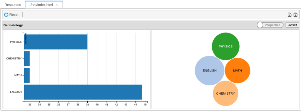
Submitting this job to the local cluster, we can browse the Visualizations by going over to the workunit’s ‘Resources’ tab.

And, we have plots!

TextMate Grammars

The current Grammar that is being used is from the Javascript version, and is a bit finicky. When it was being set up, I used an approach similar to modelling a CFG – I mapped the ANTLR statements over to syntax mapping rules. That’s not the best idea.

I lookup and read a few grammars that were present for existing languages, giving some extra time to SQL. Turns out, most of them do not use that method above (Not a surprise to anyone).

When doing syntax highlighting, the developer also needs feedback as its being typed. If you wait for the whole statement to match, the whole statement will be in plain white until the ending ‘;’.

A much better way, is to recognize specific parts of the language, fast, and colour them accordingly.

Since HSQL has a lot of tokens, this is good and syntax highlighting can be done pretty effectively. Adding in the tokens for the language, we see some good highlighting, which the user can take advantage of as they are typing.

That took a while to get right, and as a result, this solves too issues at mind:

  1. Performance and complexity: The regexes and captures were difficult, long and annoying to read. By just identifying and colouring the tokens, the grammar is much simpler, and easy to read (and maintain).
  2. Tying into the ANTLR grammar: As the earlier TextMate grammar was identifying whole statements, the two grammars needed to be completely in sync, which is difficult considering the fact that the language is being actively worked on. Identifying token-wise simplifies things, and as we no longer dependent on the grammar, the grammar can be worked on and the syntax highlighting will still work very well. Only every now and then, new keywords that will be a part of the language need to be added into the TextMate grammar.

Wrapping up

Week 6 completes, and so do the midterm goals that we had planned for. The plan for the next week is roughly:

  1. Decide on the plan ahead
  2. Fix VSCode extension related bugs: Due to some breakage due to the addition of the File Providers in earlier weeks, quite a few bugsfixes have to be done for the HSQL extension.
  3. Add in DISTRIBUTE BY to Select – This would correspond to DISTRIBUTE in ECL
  4. Investigate grammar for WRITE TO variant of the OUTPUT statement for writing to files.
Categories
HSQL

Week 5: Imports, more imports and plots

This week’s plan is to work on imports, as a step leading to the implementation of the PLOT statement. The idea is to be able to locate ECL imports, and hint to the compiler what is contained in an ECL file.

DHSQL

An idea inspired by the relationship between javascript and TypeScript, the idea is to have “type definition” for ECL files if we need to mention what is contained in these files.

Let’s consider an example for an ECL file, a.ecl:

export a:= MODULE
  export t1:= DATASET([{1,2},{3,4},{4,5}],{integer c1,integer c2});
  export t2:=DATASET([{1,3},{3,5},{3,5}],{integer c3,integer c4});
END;

Essentially, two datasets being exported. Currently, HSQl resolves it to an AnyModule, meaning that it won’t offer any type suggestions for the module when imported. To solve this, we can add in a a.dhsql in the same folder, which is intended to look something like this:

declare t1 as TABLE (integer c1,integer c2);
declare t2 as TABLE (integer c3,integer c4);

Now, when doing an import a;, HSQL can lookup this definition file, and use it to get an idea of what has been defined in the ECL file. Now, implementing this requires another piece of work – import resolution and priority.

Import resolution and priority

ECL has an interesting property where a folder may also be imported, and it is treated as a module, where all its children files/folders are members of that module. Although beyond our scope (and priority) as of now, its important to remember this as many modules use this structure too.

Now, considering all this, when we say import a; it can refer to 5 different sources:

  1. HSQL – a.hsql
  2. DHSQL – a.dhsql
  3. ECL – a.ecl
  4. A plain folder – a/...

It seems that ECL files are preferred over folders, and for our case, we need to refer to the DHSQL file if present (and of course .hsql files get more priority). So this gives us a nice order to refer to files in our system.

Adding to this, the ECL compiler itself has an order for scanning directories. It searches the standard libraries, the bundles and then the current directory as required. As we need to replicate this order too, to find the order, the idea is to first query eclcc about these paths before obtaining them. Once we have these , we can start looking at the paths in this general order:

  1. Standard Library includes – This essentially includes the standard library.
  2. ECL Bundles – This includes any bundles that have been installed by the user.
  3. Current directory – This includes imports from the current directory.

This gives us a good way to search for files. However, we also need to add some additional layers to this, to cater to some important features:

  1. A standard library type definitions layer: placed right at the top, the idea is to add definitions for standard library functions in this way.
  2. Memory map: Placed above the current directory file map (or replacing it), this can perform as –
    1. An override for on-disk files. This is common for files that are open in an IDE, but are unsaved. In this case, these files are open for use.
    2. An in-memory store of files – This is useful for use if HSQL needs to be used as a compile server.

DHSQL works!

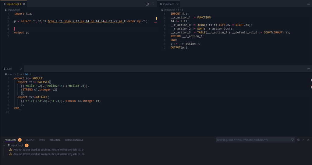
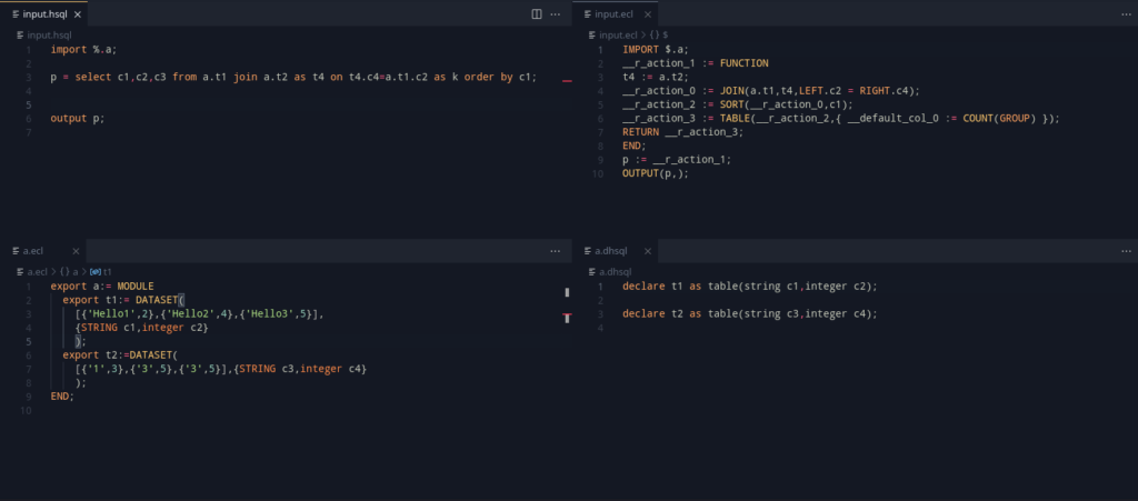
After adding in the AST Generator, we have to take slight care that Output generation is skipped for DHSQL files (because it is a declaration file). So after adding this in, we can have much better queries. Last week’s examples were shown with patched in code that would show warnings otherwise. Let’s see what this addition brings us:

Before: Warnings about types – HSQL can’t help in detecting errors
After: Now that we have a DHSQL File, HSQL can tell what’s wrong and right about the table

Nice! Now when a select statement doesn’t give any errors, it should ideally work without any issues really in ECL too, given that the DHSQL file is correct.

DHSQL – Declaring Plots

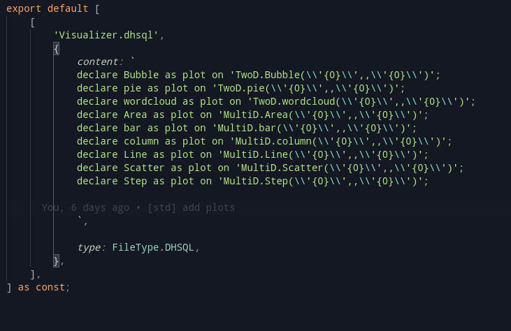
As a precursor to making the plot statement, the idea is to have DHSQL files emit methods for plots. Let’s take a look at the syntax that’s in my mind.

Consider we are making Visualizer.dhsql, the idea is to make it somewhat like this:

declare Bubble as plot on 'TwoD.Bubble(\'{0}\',,\'{0}\')';

I think the statement itself is self explanatory with enough familiarity to the Visualizer Bundle. The idea, is to supply HSQL with the little bit of information/macro on what it should call. {0} is the plot name here, and will be automatically supplied to it.

Picking up from the previous topic, we can add in plot methods by injecting a Visualizer.dhsql.

Lots of plot methods!

Now, when we import Visualizer, it should pull in these methods onto our Variable table list. But before that, there’s one more thing to do.

Auto Imports

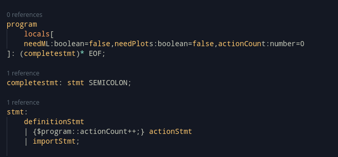
Auto imports are the best way to simplify any language. Here, the idea is to automatically pull in Visualizer, and later ML_Core as we use their respective statements. Last time around, we set values in the Parser module and retrieved them. This had the disadvantage of needing to pull them out of the parser and push them back into the visitor where the processing is happening. An easier way, is using ANTLR locals. These are dynamically scoped variables that can be accessed by any child rule (read as: really really useful if you need to just set some flags).

Locals, declaring and referencing

As these are members of the ProgramContext type itself, it becomes super easy to reference and get the values out during visiting (and skips some hoops that we had).

Where does this bring us? To auto imports. If the flags are set by the time we start visiting, that means we can be assured that there’s a plot statement somewhere in the program (Because parsing is over, and this is set during parsing).

The culmination of the above work

Finally, it became possible to test the workings.
Although AST and codegen are not present at this point, it simply means the plot statement code will not be generated.

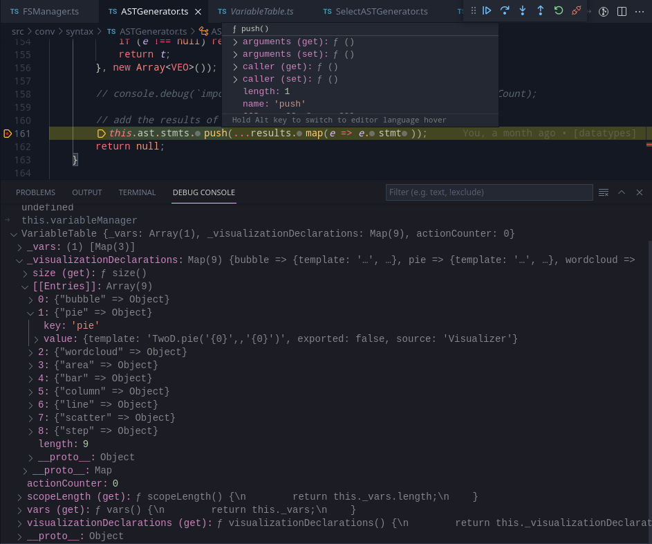
Using a debugger, we can break just before the statements are pushed out from the AST Generator. And the results are promising!

Look at all the plot methods!

With this, we have a general idea on how the PLOT statement will be represented in AST. With this, I stopped to continue in the next week.

Wrapping up – Week 6

Week 6 is the midweek. The goal was to set up atleast 2 plot statements, but I can comfortably say the whole set we showed above will be possible. So, for Week 6, the idea is to finish:

  1. Plot codegen and output – This involves using the template and generating the PLOT statement.
  2. Add the new PLOT and OUTPUT statement to the VSCode Textmate grammar. This requires some research into how Textmate grammars are actually made in VSCode (we’ve been doing a lot of straight implementations so far)
Categories
HSQL

Week 4: Working towards SELECT

This week’s work is planned exclusively around getting select to work; its a huge part of the language. The decision, was to use FUNCTIONS, to emulate a SELECT. Why? Because functions in ECL have their own scoping, and local variables declared there, will be usable outside the scope of the function. However, a function cannot shadow variables that exist. Selects, have aliases, which can perfectly be matched by local function-scoped definitions, and can help skip the entire process of defining “formal” (visible variable name) and the “behind the scenes” variable names.

The idea

The idea is a simple 6 step process:

  1. Create a function and assign it to a value
  2. Enumerate all the sources that have been changed, or need processing – JOINS, select in select and aliases.
    1. JOINS – do a join
    2. select in select – follow this procedure and assign it to its alias
    3. Aliases – assign the original value to the alias
  3. Now, take all the sources, and join them all.
  4. Take last generated variable and then do the following in order
    1. Where – apply filter
    2. sort – sort
    3. group and column filters – table
    4. limit offset – choosen
    5. distinct – dedup all
  5. Wrap this whole block of statements in a function, returning the last generated variable.
  6. The variable assigned to the function on step 5, can now be the result. (assign it or just use it as an action)

From

The current syntax supports three kinds of data sources:

  1. Select statements – The statements can have a SELECT statement as part of a table source. To ease our worries and pain, SQL mandates that such sources have a defined alias. Whew. The idea for these, is to run this algorithm (read as: thank god recursion exists) for generating the select statement, and assign it to this select statement.
  2. Table Definitions – The statements can refer to table definitions and also have an alias. This is a simple case of a redefinition if a reassignment happens.
  3. Joins – Joins are a part of SQL, where there is a specific join type, and an expression that helps the join. Unfortunately joins do not have an alias, and this brings us to an annoyance – we need to force create an alias and let the user know in that case.

The multiple datasets are then joined, and the result variable is put on a stack. What happens from here on, is based on the order above. the top of the stack’s variable is used to generate a new variable, which is then placed on the top. This keeps the optional parts actually optional and generates the definitions only as necessary.

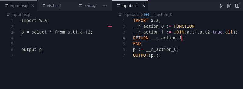
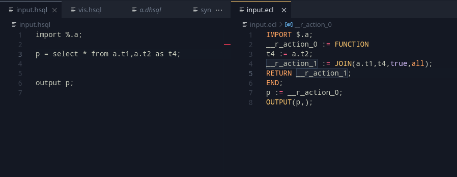
Implementing the from part, we get some interesting outputs that work well!

Selecting from multiple tables joins them
Alias reassigns them accordingly

From here, the rest of the statements can be added in. The column filtering is important, as they are the only other mandatory part of select.

The rest of SELECT

The rest of the select, uses the last generated variable, and creates a new one.

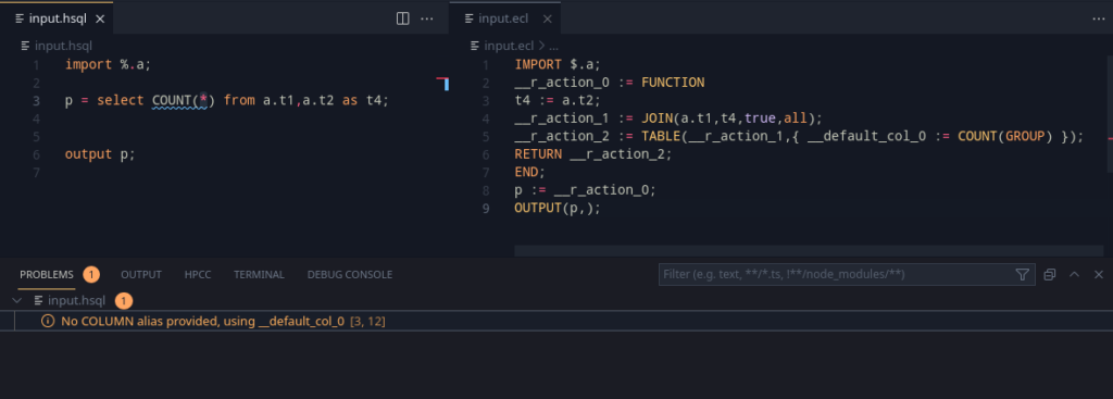
Making some of them, here’s what we get:

The last example, but completed
Columns must always have an alias, as ECL’s naming rules are a bit too difficult for us.
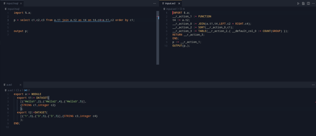
What about sorting? Covered as well!
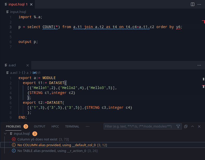
An error: We track the datatypes as we create them, so since we know t1 and t2 dont have y6, the combined result can’t have them as well (I’m monkeypatching the data types for a1 and a2 for testing here, it will be implemented soon)

Looking at the grammar, the ORDER BY, GROUP BY, WHERE was added in. That’s a lot of querying capabilities as part of one sentence.

The having query segment was considered, but dropped as it can be done by two queries (Another where after the group by).

Winding up

This took a good part of the week. Adding the support code did take a bit of the time, but this allows us to use the most important part of SQL. The plan for the upcoming week is as follows:

  1. Start looking at import resolution. Imports need to be vetted to make sure that there exists atleast a folder, .ecl file or a HSQL file.
  2. HSQL might need a way to do auto imports for certain core modules such as Visualizer and ML_Core (for Plots and for Machine learning related statements). This should help with ease-of-use.
  3. Plots – The plot statement is another important objective as visualizing is an import usecase for HSQL. The idea is to support basic and important visualization methods, and try to find out if there’s a way that other modules can integrate into HSQL and add to more plot methods.